In this section we describe two more involved examples of using an IPython cluster to perform a parallel computation. In these examples, we will be using IPython’s “pylab” mode, which enables interactive plotting using the Matplotlib package. IPython can be started in this mode by typing:
ipython --pylab
at the system command line.
In this example we would like to study the distribution of digits in the number pi (in base 10). While it is not known if pi is a normal number (a number is normal in base 10 if 0-9 occur with equal likelihood) numerical investigations suggest that it is. We will begin with a serial calculation on 10,000 digits of pi and then perform a parallel calculation involving 150 million digits.
In both the serial and parallel calculation we will be using functions defined in the pidigits.py file, from the IPython examples. These functions provide basic facilities for working with the digits of pi and can be loaded into IPython by locating pidigits.py, and doing:
In [1]: run pidigits.py
For the serial calculation, we will use SymPy to calculate 10,000 digits of pi and then look at the frequencies of the digits 0-9. Out of 10,000 digits, we expect each digit to occur 1,000 times. While SymPy is capable of calculating many more digits of pi, our purpose here is to set the stage for the much larger parallel calculation.
In this example, we use two functions from pidigits.py: one_digit_freqs() (which calculates how many times each digit occurs) and plot_one_digit_freqs() (which uses Matplotlib to plot the result). Here is an interactive IPython session that uses these functions with SymPy:
In [7]: import sympy

In [8]: pi = sympy.pi.evalf(40)

In [9]: pi
Out[9]: 3.141592653589793238462643383279502884197

In [10]: pi = sympy.pi.evalf(10000)

In [11]: digits = (d for d in str(pi)[2:])  # create a sequence of digits

In [12]: run pidigits.py  # load one_digit_freqs/plot_one_digit_freqs

In [13]: freqs = one_digit_freqs(digits)

In [14]: plot_one_digit_freqs(freqs)
Out[14]: [<matplotlib.lines.Line2D object at 0x18a55290>]
The resulting plot of the single digit counts shows that each digit occurs approximately 1,000 times, but that with only 10,000 digits the statistical fluctuations are still rather large:
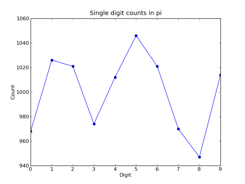
It is clear that to reduce the relative fluctuations in the counts, we need to look at many more digits of pi. That brings us to the parallel calculation.
Calculating many digits of pi is a challenging computational problem in itself. Because we want to focus on the distribution of digits in this example, we will use pre-computed digit of pi from the website of Professor Yasumasa Kanada at the University of Tokyo (http://www.super-computing.org). These digits come in a set of text files (ftp://pi.super-computing.org/.2/pi200m/) that each have 10 million digits of pi.
For the parallel calculation, we download these files to the compute nodes, and use one file per node. To make things a little more interesting we will calculate the frequencies of all 2 digits sequences (00-99) and then plot the result using a 2D matrix in Matplotlib.
The overall idea of the calculation is simple: each IPython engine will compute the two digit counts for the digits in a single file. Then in a final step the counts from each engine will be added up. To perform this calculation, we will need two top-level functions from pidigits.py:
    """
    Read digits of pi from a file and compute the 2 digit frequencies.
    """
    d = txt_file_to_digits(filename)
    freqs = two_digit_freqs(d)
    return freqs

def reduce_freqs(freqlist):
    """
    Add up a list of freq counts to get the total counts.
    """
    allfreqs = np.zeros_like(freqlist[0])
    for f in freqlist:
        allfreqs += f
    return allfreqs
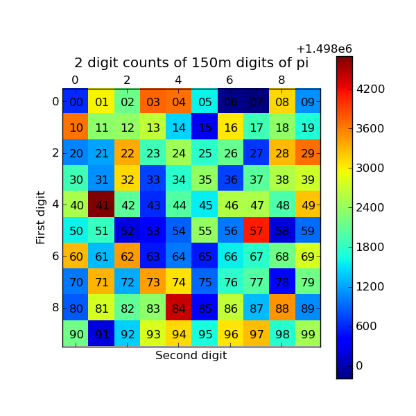
We will also use the plot_two_digit_freqs() function to plot the results. The resulting plot generated by Matplotlib is shown below. The colors indicate which two digit sequences are more (red) or less (blue) likely to occur in the first 150 million digits of pi. We clearly see that the sequence “41” is most likely and that “06” and “07” are least likely. Further analysis would show that the relative size of the statistical fluctuations have decreased compared to the 10,000 digit calculation.
An option is a financial contract that gives the buyer of the contract the right to buy (a “call”) or sell (a “put”) a secondary asset (a stock for example) at a particular date in the future (the expiration date) for a pre-agreed upon price (the strike price). For this right, the buyer pays the seller a premium (the option price). There are a wide variety of flavors of options (American, European, Asian, etc.) that are useful for different purposes: hedging against risk, speculation, etc.
Much of modern finance is driven by the need to price these contracts accurately based on what is known about the properties (such as volatility) of the underlying asset. One method of pricing options is to use a Monte Carlo simulation of the underlying asset price. In this example we use this approach to price both European and Asian (path dependent) options for various strike prices and volatilities.
The function price_options() in mcpricer.py implements the basic Monte Carlo pricing algorithm using the NumPy package and is shown here:
def price_options(S=100.0, K=100.0, sigma=0.25, r=0.05, days=260, paths=10000):
    """
    Price European and Asian options using a Monte Carlo method.

    Parameters
    ----------
    S : float
        The initial price of the stock.
    K : float
        The strike price of the option.
    sigma : float
        The volatility of the stock.
    r : float
        The risk free interest rate.
    days : int
        The number of days until the option expires.
    paths : int
        The number of Monte Carlo paths used to price the option.

    Returns
    -------
    A tuple of (E. call, E. put, A. call, A. put) option prices.
    """
    import numpy as np
    from math import exp,sqrt

    h = 1.0/days
    const1 = exp((r-0.5*sigma**2)*h)
    const2 = sigma*sqrt(h)
    stock_price = S*np.ones(paths, dtype='float64')
    stock_price_sum = np.zeros(paths, dtype='float64')
    for j in range(days):
        growth_factor = const1*np.exp(const2*np.random.standard_normal(paths))
        stock_price = stock_price*growth_factor
        stock_price_sum = stock_price_sum + stock_price
    stock_price_avg = stock_price_sum/days
    zeros = np.zeros(paths, dtype='float64')
    r_factor = exp(-r*h*days)
    euro_put = r_factor*np.mean(np.maximum(zeros, K-stock_price))
    asian_put = r_factor*np.mean(np.maximum(zeros, K-stock_price_avg))
    euro_call = r_factor*np.mean(np.maximum(zeros, stock_price-K))
    asian_call = r_factor*np.mean(np.maximum(zeros, stock_price_avg-K))
    return (euro_call, euro_put, asian_call, asian_put)