To run this code in parallel, we will use IPython’s LoadBalancedView class, which distributes work to the engines using dynamic load balancing. This view is a wrapper of the Client class shown in the previous example. The parallel calculation using LoadBalancedView can be found in the file mcpricer.py. The code in this file creates a LoadBalancedView instance and then submits a set of tasks using LoadBalancedView.apply() that calculate the option prices for different volatilities and strike prices. The results are then plotted as a 2D contour plot using Matplotlib.
#!/usr/bin/env python
"""Run a Monte-Carlo options pricer in parallel."""

#-----------------------------------------------------------------------------
# Imports
#-----------------------------------------------------------------------------

import sys
import time
from IPython.parallel import Client
import numpy as np
from mcpricer import price_options
from matplotlib import pyplot as plt

#-----------------------------------------------------------------------------
# Setup parameters for the run
#-----------------------------------------------------------------------------

def ask_question(text, the_type, default):
    s = '%s [%r]: ' % (text, the_type(default))
    result = raw_input(s)
    if result:
        return the_type(result)
    else:
        return the_type(default)

cluster_profile = ask_question("Cluster profile", str, "default")
price = ask_question("Initial price", float, 100.0)
rate = ask_question("Interest rate", float, 0.05)
days = ask_question("Days to expiration", int, 260)
paths = ask_question("Number of MC paths", int, 10000)
n_strikes = ask_question("Number of strike values", int, 5)
min_strike = ask_question("Min strike price", float, 90.0)
max_strike = ask_question("Max strike price", float, 110.0)
n_sigmas = ask_question("Number of volatility values", int, 5)
min_sigma = ask_question("Min volatility", float, 0.1)
max_sigma = ask_question("Max volatility", float, 0.4)

strike_vals = np.linspace(min_strike, max_strike, n_strikes)
sigma_vals = np.linspace(min_sigma, max_sigma, n_sigmas)

#-----------------------------------------------------------------------------
# Setup for parallel calculation
#-----------------------------------------------------------------------------

# The Client is used to setup the calculation and works with all
# engines.
c = Client(profile=cluster_profile)

# A LoadBalancedView is an interface to the engines that provides dynamic load
# balancing at the expense of not knowing which engine will execute the code.
view = c.load_balanced_view()

# Initialize the common code on the engines. This Python module has the
# price_options function that prices the options.

#-----------------------------------------------------------------------------
# Perform parallel calculation
#-----------------------------------------------------------------------------

print "Running parallel calculation over strike prices and volatilities..."
print "Strike prices: ", strike_vals
print "Volatilities: ", sigma_vals
sys.stdout.flush()

# Submit tasks to the TaskClient for each (strike, sigma) pair as a MapTask.
t1 = time.time()
async_results = []
for strike in strike_vals:
    for sigma in sigma_vals:
        ar = view.apply_async(price_options, price, strike, sigma, rate, days, paths)
        async_results.append(ar)

print "Submitted tasks: ", len(async_results)
sys.stdout.flush()

# Block until all tasks are completed.
c.wait(async_results)
t2 = time.time()
t = t2-t1

print "Parallel calculation completed, time = %s s" % t
print "Collecting results..."

# Get the results using TaskClient.get_task_result.
results = [ar.get() for ar in async_results]

# Assemble the result into a structured NumPy array.
prices = np.empty(n_strikes*n_sigmas,
    dtype=[('ecall',float),('eput',float),('acall',float),('aput',float)]
)

for i, price in enumerate(results):
    prices[i] = tuple(price)

prices.shape = (n_strikes, n_sigmas)
strike_mesh, sigma_mesh = np.meshgrid(strike_vals, sigma_vals)

print "Results are available: strike_mesh, sigma_mesh, prices"
print "To plot results type 'plot_options(sigma_mesh, strike_mesh, prices)'"

#-----------------------------------------------------------------------------
# Utilities
#-----------------------------------------------------------------------------

def plot_options(sigma_mesh, strike_mesh, prices):
    """
    Make a contour plot of the option price in (sigma, strike) space.
    """
    plt.figure(1)

    plt.subplot(221)
    plt.contourf(sigma_mesh, strike_mesh, prices['ecall'])
    plt.axis('tight')
    plt.colorbar()
    plt.title('European Call')
    plt.ylabel("Strike Price")

    plt.subplot(222)
    plt.contourf(sigma_mesh, strike_mesh, prices['acall'])
    plt.axis('tight')
    plt.colorbar()
    plt.title("Asian Call")

    plt.subplot(223)
    plt.contourf(sigma_mesh, strike_mesh, prices['eput'])
    plt.axis('tight')
    plt.colorbar()
    plt.title("European Put")
    plt.xlabel("Volatility")
    plt.ylabel("Strike Price")

    plt.subplot(224)
    plt.contourf(sigma_mesh, strike_mesh, prices['aput'])
    plt.axis('tight')
    plt.colorbar()
    plt.title("Asian Put")
    plt.xlabel("Volatility")

if __name__ == '__main__':
    plot_options(sigma_mesh, strike_mesh, prices)
    plt.show()
To use this code, start an IPython cluster using ipcluster, open IPython in the pylab mode with the file mcdriver.py in your current working directory and then type:
In [7]: run mcdriver.py
Submitted tasks:  [0, 1, 2, ...]
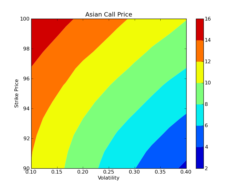
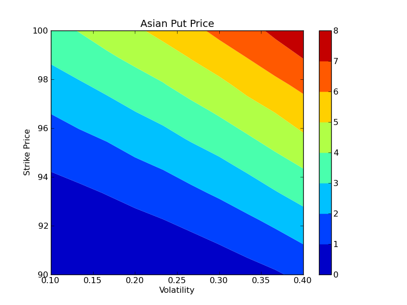
Once all the tasks have finished, the results can be plotted using the plot_options() function. Here we make contour plots of the Asian call and Asian put options as function of the volatility and strike price:
In [8]: plot_options(sigma_vals, K_vals, prices['acall'])

In [9]: plt.figure()
Out[9]: <matplotlib.figure.Figure object at 0x18c178d0>

In [10]: plot_options(sigma_vals, K_vals, prices['aput'])
These results are shown in the two figures below. On a 8 core cluster the entire calculation (10 strike prices, 10 volatilities, 100,000 paths for each) took 30 seconds in parallel, giving a speedup of 7.7x, which is comparable to the speedup observed in our previous example.